Worked Examples

This page introduces the main ways to use pygenstates. The examples are adapted from the worked notebooks in the repository’s examples folder. The solver can be applied to a variety of systems, but several examples use circuit QED notation because that is one of the motivating applications.

The continuous solver represents Hamiltonians of the form

\[\left[-\sum_i k_{ii}\frac{\partial^2}{\partial x_i^2} -\sum_{i<j} k_{ij}\frac{\partial^2}{\partial x_i\partial x_j} +U(x)\right]\psi=E\psi.\]

where U is a Python callable representing the potential. The diagonal kinetic coefficients \(k_{ii}\) are passed with k_diag. Cross couplings between generalized momenta are included with coefficients \(k_{ij}\) and are passed with k_cross. The first examples set k_cross=[], which drops these terms.

Most examples call eigensolver with the same basic arguments:

U

Potential function. It accepts one array argument per coordinate.

N

Number of grid points in each coordinate direction, including boundary points.

domain

Coordinate bounds for each direction.

k_diag

Coefficients multiplying the diagonal second-derivative terms.

Enum

Number of eigenpairs to compute.

k_cross

Optional coefficients multiplying the mixed derivative terms.

Additional keyword arguments such as sigma=0 are passed through to SciPy’s sparse eigensolvers. sigma=0 requests eigenvalues near zero using shift-invert mode. For the full list of optional arguments, refer to the API reference.

Imports

import numpy as np
import matplotlib.pyplot as plt

import pygenstates as eg

One-Dimensional Harmonic Oscillator

The one-dimensional harmonic oscillator is a useful first example. For

\[H=-E_m\frac{d^2}{dx^2}+E_u x^2,\]

where x is a dimensionless generalized coordinate, E_m sets the kinetic energy scale, and E_u sets the harmonic potential energy scale, the exact eigenvalues are

\[E_n=\sqrt{E_mE_u}(2n+1),\qquad n=0,1,2,\ldots.\]

E_m = 1
E_u = 1

U_ho_1d = lambda x: E_u*x**2

vals, vecs, xlists = eg.eigensolver(
    U_ho_1d,
    N=[801],
    domain=[(-6, 6)],
    k_diag=[E_m],
    Enum=5,
    which="SA",  # finds smallest algebraic eigenvalues
)

exact_vals = np.array([np.sqrt(E_m*E_u)*(2*n + 1) for n in range(5)])
print("Numerical eigenvalues:", vals)
print("Exact eigenvalues:    ", exact_vals)
print("Errors:               ", vals - exact_vals)

The return value is (vals, vecs, xlists). vals contains the eigenvalues, vecs contains the eigenvectors on the full grid, and xlists contains the coordinate arrays used to construct the grid.

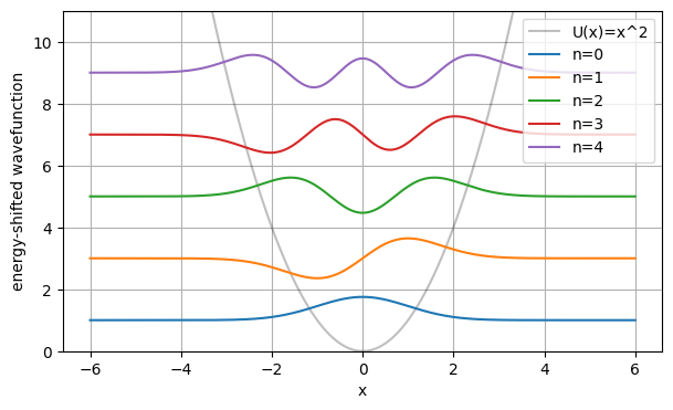
The first five harmonic-oscillator eigenfunctions, shifted by their eigenvalues and plotted over \(U(x)=x^2\).

Two-Dimensional Harmonic Oscillator

The same interface extends to multiple spatial coordinates by passing a multi-entry N, domain, and k_diag. For

\[H=-E_{mx}\frac{\partial^2}{\partial x^2} -E_{my}\frac{\partial^2}{\partial y^2} +E_{ux}x^2+E_{uy}y^2,\]

the separable energy spectrum is

\[E_{n_x,n_y}=\sqrt{E_{mx}E_{ux}}(2n_x+1) +\sqrt{E_{my}E_{uy}}(2n_y+1).\]

The example below uses all four energy scales equal to one.

E_ms = [1, 1]
E_us = [1, 1]

U_ho_2d = lambda x, y: E_us[0]*x**2 + E_us[1]*y**2

vals, vecs, xlists = eg.eigensolver(
    U_ho_2d,
    N=[101, 101],
    domain=[(-4, 4), (-4, 4)],
    k_diag=E_ms,
    Enum=6,
    which="SA",
)

exact_2d = sorted([
    np.sqrt(E_ms[0]*E_us[0])*(2*nx + 1)
    + np.sqrt(E_ms[1]*E_us[1])*(2*ny + 1)
    for nx in range(4)
    for ny in range(4)
])[:6]
print("Numerical eigenvalues:", vals)
print("Exact eigenvalues:    ", np.array(exact_2d))
print("Errors:               ", vals - np.array(exact_2d))

x, y = xlists
X, Y = np.meshgrid(x, y, indexing="ij")

plt.contourf(X, Y, np.real(vecs[1]), levels=40, cmap="RdBu_r")
plt.gca().set_aspect("equal")
plt.xlabel("x")
plt.ylabel("y")
plt.title(f"State 1, E={vals[1]:.5f}")
plt.colorbar(label=r"$\psi(x,y)$")
plt.show()

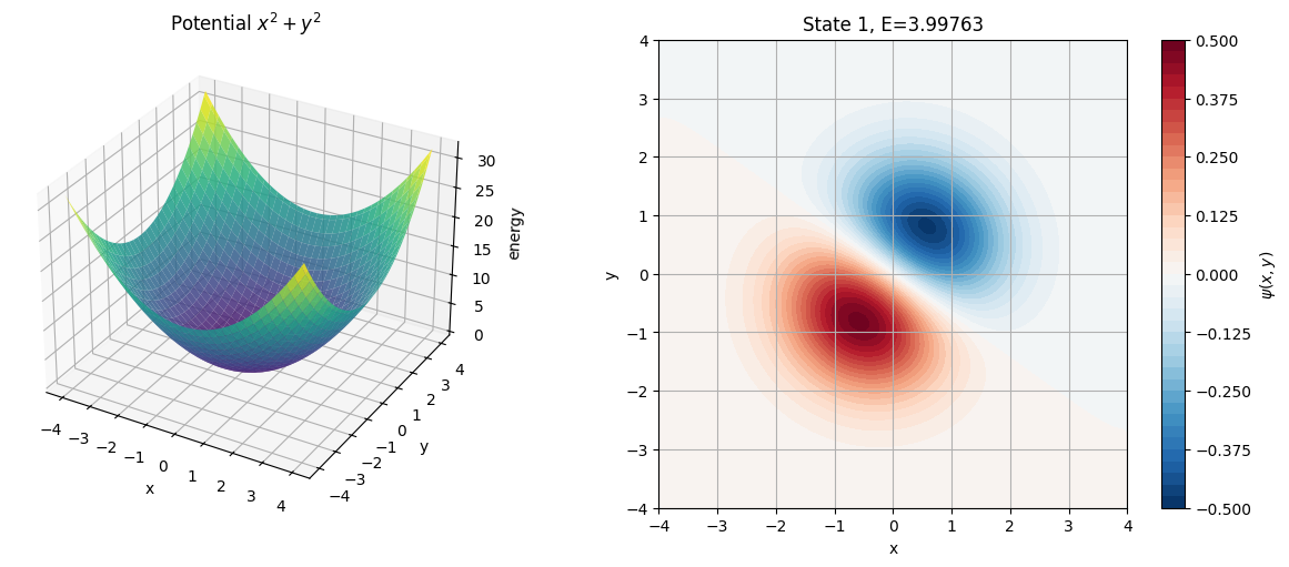
A 2D harmonic-oscillator solve, showing the potential surface and one eigenfunction on the tensor-product grid.

Hydrogen Atom on a Cartesian Grid

The finite-difference backend supports dimensions beyond the one-, two-, and three-dimensional cases shown here. This example solves the hydrogen atom directly on a 3D Cartesian grid, using angstroms for coordinates and electron-volts for energies:

\[H=-\frac{\hbar^2}{2m_e}\nabla^2-\frac{e^2}{4\pi\epsilon_0 r}.\]

To keep the example reasonably quick and stable, the Coulomb singularity at r=0 is clipped at a small radius. The potential is also shifted upward by a constant so that the targeted bound-state energies lie near zero during the solve. That offset is subtracted from the eigenvalues afterward.

q_e = 1.60217663e-19
m_e = 9.1093837e-31
eps0 = 8.85418782e-12
hbar = 1.054571817e-34

r_cutoff = 0.2
k_HA_2eV = hbar**2 / (2 * m_e * q_e * 1e-20)
offset = q_e * 1e10 / (r_cutoff * eps0 * 4 * np.pi)

def U_hydrogen_shifted(x, y, z):
    r = np.sqrt(x*x + y*y + z*z)
    r_eff = np.maximum(r, r_cutoff)
    return -q_e * 1e10 / (r_eff * eps0 * 4 * np.pi) + offset

vals, vecs, xlists = eg.eigensolver(
    U_hydrogen_shifted,
    N=[41, 41, 41],
    domain=[(-10, 10), (-10, 10), (-10, 10)],
    k_diag=[k_HA_2eV, k_HA_2eV, k_HA_2eV],
    Enum=5,
    method="finite_difference",
    which="SA",
)

hydrogen_vals = vals - offset
expected = np.array([-13.6 / n**2 for n in [1, 2, 2, 2, 2]])

print("Numerical bound energies, eV:", hydrogen_vals)
print("Reference pattern, eV:       ", expected)
print("Errors, eV:                  ", hydrogen_vals - expected)

Increasing the grid size and domain improves convergence, at the cost of a larger sparse eigenproblem.

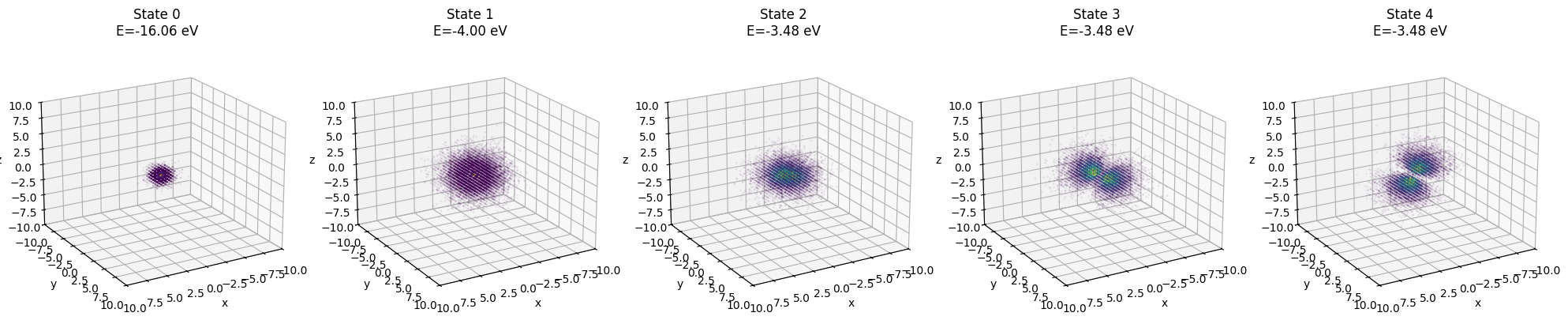
Probability-density samples for the first five hydrogen states from the direct 3D Cartesian-grid solve.

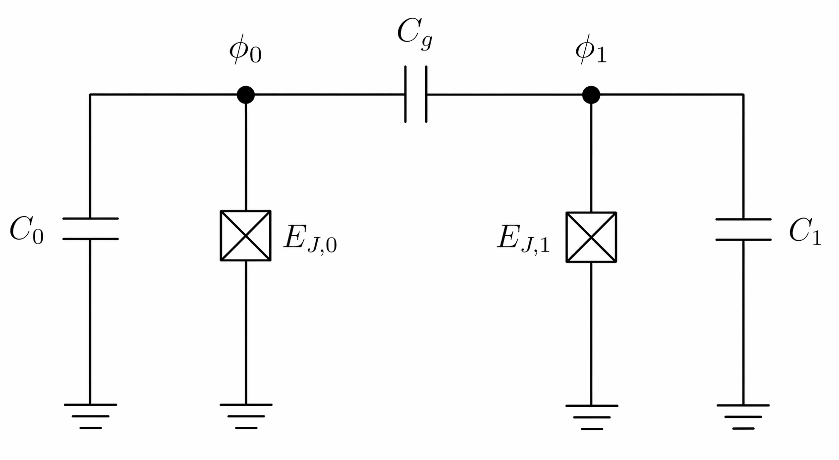
Continuous-Discrete Coupling

Ceigensolver extends the continuous spatial problem with a finite-dimensional discrete basis. The returned wavefunctions have shape (Enum, M, *N), where M is the dimension of the discrete basis.

This is useful for Hamiltonians written in a mixture of discrete and continuous bases. The following circuit-QED example couples a continuous harmonic oscillator coordinate to a two-level subsystem.

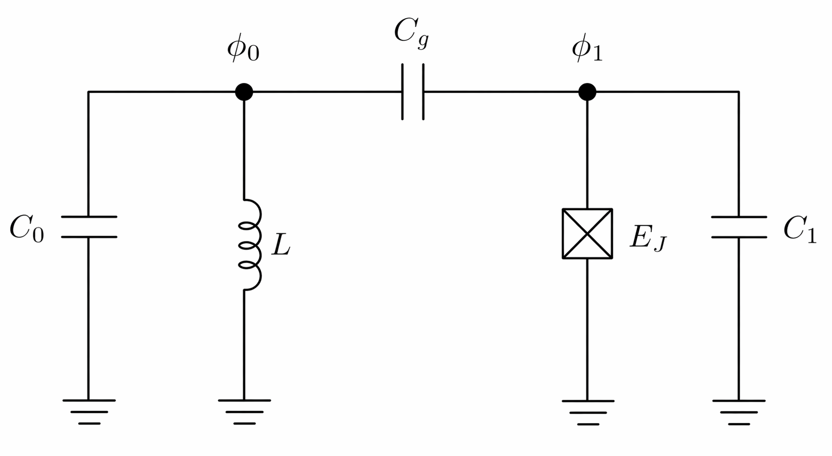
Circuit model for a continuous oscillator coupled to a qubit-like two-level subsystem.

\[H = H_0 + H_1 + H_c,\]

where

\[\begin{split}H_0=-E_C\frac{d^2}{d\phi^2}+E_L\phi^2, \qquad H_1=\begin{pmatrix}0&0\\0&E_q\end{pmatrix}.\end{split}\]

The oscillator Hamiltonian uses \(E_C=2e^2/C_0\) and \(E_L=(\hbar/2e)^2/(2L)\). The two-level subsystem has approximate transition energy \(E_q\approx\sqrt{E_{C,1}E_J}-E_{C,1}/4\). The coupling capacitor gives the derivative coupling

\[\begin{split}H_c=\begin{pmatrix} 0 & -E_g\frac{d}{d\phi}\\ E_g\frac{d}{d\phi} & 0 \end{pmatrix},\end{split}\]

where \(E_g\approx 4e^2 C_g n_{J,\mathrm{zpf}}/(C_0 C_1)\) for \(C_g\ll C_0,C_1\) and \(n_{J,\mathrm{zpf}}=(E_J/(8E_{C,1}))^{1/4}\).

The derivative coupling is supplied with k_coup. Linear position couplings of the form \(E_g\phi_0\phi_1\) can be supplied with v_coup.

For more than one continuous coordinate, pass a dictionary keyed by coordinate axis. For example, k_coup={0: K_phi, 1: K_theta} applies one discrete coupling matrix to derivatives along coordinate 0 and another to derivatives along coordinate 1.

Couplings can also be written as a list of pair dictionaries, one dictionary per continuous coordinate. This is often the most direct representation of

\[H_c=\sum_i \sum_{n>m} \left(-k_{c,i,nm}\frac{d}{dx_i}+v_{c,i,nm}x_i\right) |n\rangle\langle m|+\mathrm{h.c.}\]

For example:

k_coup = [
    {(0, 1): E01_phi, (1, 2): E12_phi},  # derivative couplings along axis 0
    {(0, 2): E02_theta},                 # derivative couplings along axis 1
]

v_coup = [
    {(0, 1): V01_phi},
    {},
]

For derivative couplings, the conjugate partner is filled with the sign needed to produce a Hermitian total derivative operator. For position couplings, the conjugate partner is filled in the usual Hermitian way.

The full coupled wavefunction returned by the solver has components \(\Psi_i(\phi)=\langle \phi,i|\Psi\rangle\), subject to the normalization \(\int\sum_i|\Psi_i(\phi)|^2\,d\phi=1\). With \(\hbar=1\), the oscillator level spacing for this convention is \(2\sqrt{E_CE_L}\). The example below chooses E_q to match that spacing and uses a weak derivative coupling E_g.

hbar = 1.0
GHz = 1.0

E_C = hbar * (2 * np.pi * 2.0 * GHz)
E_L = hbar * (2 * np.pi * 6.0 * GHz)
E_g = hbar * (2 * np.pi * 0.05 * GHz)

omega_osc = 2.0 * np.sqrt(E_C * E_L) / hbar
E_q = hbar * omega_osc

H1 = np.array([
    [0.0, 0.0],
    [0.0, E_q],
])

vals_c, vecs_c, xlists_c = eg.Ceigensolver(
    lambda x: E_L * x**2,
    H1,
    N=[801],
    domain=[(-4, 4)],
    k_diag=[E_C],
    k_coup=E_g,
    Enum=6,
    which="SA",
)

x = xlists_c[0]
component_weight = np.sum(np.abs(vecs_c)**2, axis=2) * (x[1] - x[0])
print("Coupled eigenvalues:", np.real(vals_c))
print("Discrete component weights:", component_weight)

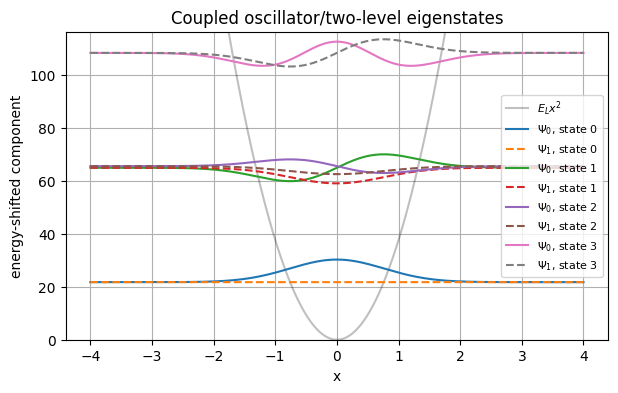
The two discrete components of several coupled eigenstates, shifted by their eigenvalues.

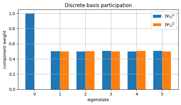
Component weights show how much each eigenstate occupies each discrete basis level.

Coupled Josephson Junctions and Mixed Derivatives

The standard solver supports mixed spatial derivative terms through k_cross. Mixed derivative terms are not present for a single particle in ordinary Cartesian coordinates, but they are useful for coupled generalized momenta, such as in circuit-QED phase coordinates. For two coupled Josephson junction phases, one possible Hamiltonian is:

Circuit model for two coupled Josephson junctions.

\[H=-E_{C,0}\frac{\partial^2}{\partial \phi_0^2} -E_{C,1}\frac{\partial^2}{\partial \phi_1^2} -E_g\frac{\partial^2}{\partial \phi_0\partial \phi_1} +U(\phi_0,\phi_1),\]

with

\[U(\phi_0,\phi_1)=E_{J,0}\left(1-\sin\phi_0\right) +E_{J,1}\left(1-\sin\phi_1\right).\]

Here \(E_{C,i}=2e^2/C_i\) and \(E_g\approx 4e^2 C_g/(C_0C_1)\) for \(C_g\ll C_0,C_1\). The diagonal kinetic terms are passed with k_diag and the mixed derivative is represented with k_cross={(0, 1): E_g}. The tuple (0, 1) indicates the coordinate pair \((\phi_0,\phi_1)\).

E_C0 = 2 * np.pi * 10.0
E_C1 = 2 * np.pi * 10.0
E_J0 = 2 * np.pi * 2.0
E_J1 = 2 * np.pi * 2.0
E_g = 2 * np.pi * 0.05

def U_phase(phi0, phi1):
    return E_J0 * (1 - np.sin(phi0)) + E_J1 * (1 - np.sin(phi1))

vals_phase, vecs_phase, phase_lists = eg.eigensolver(
    U_phase,
    N=[121, 121],
    domain=[(-np.pi, 2*np.pi), (-np.pi, 2*np.pi)],
    k_diag=[E_C0, E_C1],
    k_cross={(0, 1): E_g},
    Enum=5,
    method="finite_difference",
    which="SA",
)

print("Eigenvalues:", vals_phase)

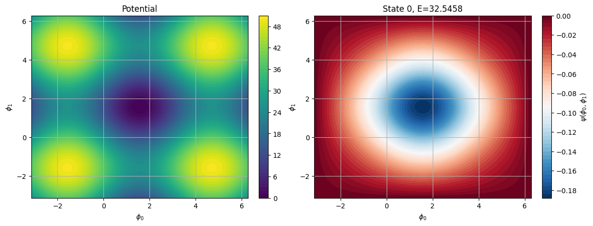
The Josephson potential and the lowest eigenfunction from a 2D solve with a mixed derivative term.

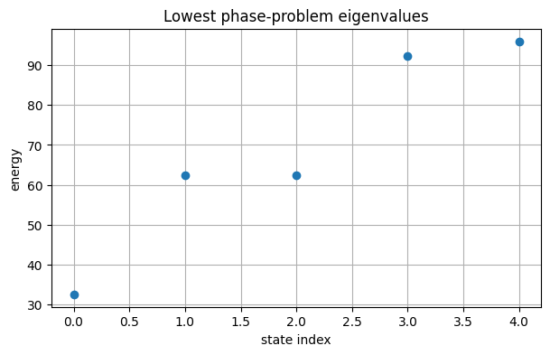
Lowest eigenvalues from the coupled phase problem.

Backend Comparison with the Airy Problem

The available backend names can be inspected programmatically:

print(eg.available_methods())

The default method is "finite_difference". The "FEM" backend uses scikit-fem and supports one-, two-, and three-dimensional problems. The finite-difference backend supports arbitrary dimension, subject to the memory and runtime cost of the resulting sparse matrix.

The Airy problem,

\[H=-k\frac{d^2}{dx^2}+|x|,\]

is a useful comparison because the decaying solutions are Airy functions. Even states are fixed by zeros of \(\mathrm{Ai}'\), and odd states are fixed by zeros of \(\mathrm{Ai}\). This gives an analytic reference for comparing the finite-difference and finite-element backends.

Discontinuous or non-differentiable potentials can reduce finite-difference accuracy, especially when high-precision eigenvectors are required. The FEM backend provides an alternative discretization that can behave better near non-smooth points.

U_abs = lambda x: np.abs(x)

common = dict(
    U=U_abs,
    N=[801],
    domain=[(-12, 12)],
    k_diag=[1],
    Enum=5,
    which="SA",
)

vals_fd, vecs_fd, xlists_fd = eg.eigensolver(
    method="finite_difference",
    **common,
)
vals_fem, vecs_fem, xlists_fem = eg.eigensolver(
    method="FEM",
    intorder=None,
    **common,
)

print("Finite difference:", vals_fd)
print("FEM:              ", vals_fem)

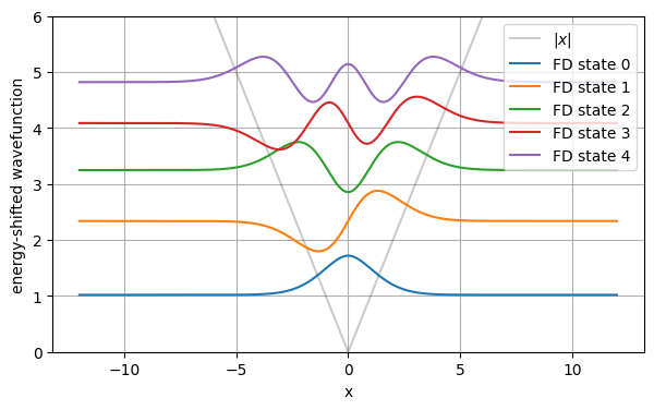
Finite-difference eigenfunctions for \(U(x)=|x|\), shifted by their eigenvalues.

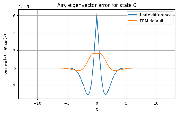
Eigenvector error against the analytic Airy solution for finite difference and FEM.

The full notebooks include the plotting setup and analytic-comparison helper functions used to generate these figures.